An
RF switch matrix is the central routing hub in many test & measurement, communication, and aerospace systems. By interconnecting multiple input and output ports through a grid of switches, it allows any input to be routed to any output — or any combination of inputs to any combination of outputs. This guide explains matrix architectures, key specifications, common applications, and how to select the right matrix for your system.
1. What Is an RF Switch Matrix?
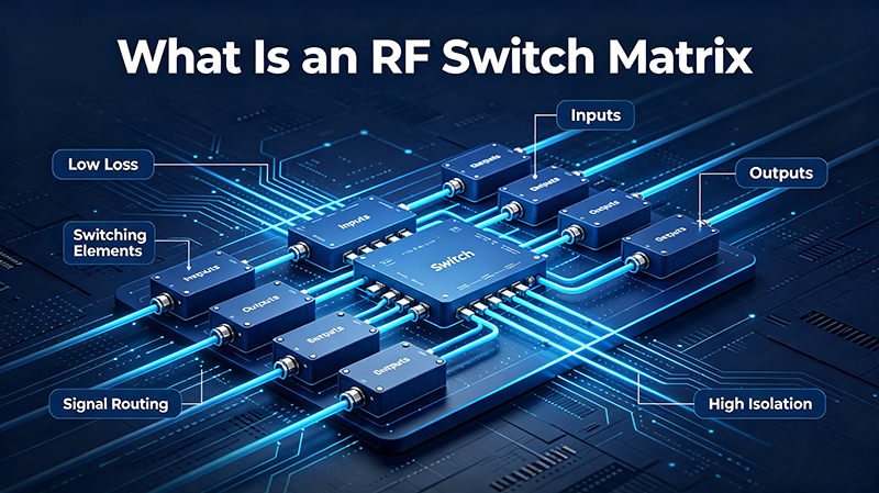
An RF switch matrix (or RF matrix switch) is a multi-port switching system that connects any input port to any output port through a configurable network of smaller switches. Where a single SPnT switch lets you pick one path among N outputs, a matrix lets you simultaneously connect M inputs to N outputs in arbitrary combinations.
For example, a 4×4 matrix contains 16 possible input-output pairs. A 32×32 matrix contains 1,024 possible paths. Matrices are used wherever signal routing flexibility is needed.
2. Three Core Architectures
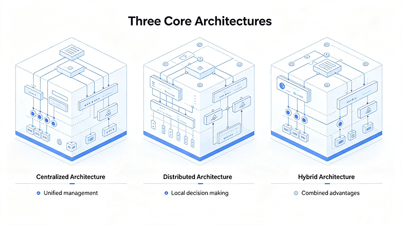
A
Blocking Matrix
Uses an SPnT switch at every input and output. Simple and low loss, but cannot connect multiple inputs to a single output. Ideal for one-to-one routing.
B
Non-Blocking Matrix
Every input can connect to every output simultaneously. Built with cross-point or multi-layer switches. More switches — more flexibility.
C
Hybrid Matrix
Combines multiple smaller matrices. Balances cost, size, and flexibility. Common in large systems (e.g. 64×64) where full non-blocking is impractical.
2.1 Blocking Matrix
A blocking matrix uses an SPnT switch at every input, with each output connected to a fixed input's SPnT. Once one input is selected, no other input can route to that output. Blocking matrices are simple, low loss, and inexpensive — but limited.
IN1 ──[SPnT]───────► OUT1
IN2 ──[SPnT]───────► OUT2
IN3 ──[SPnT]───────► OUT3
IN4 ──[SPnT]───────► OUT4
(one-to-one routing only)
2.2 Non-Blocking Matrix
A non-blocking matrix uses cross-point switches at every intersection of inputs and outputs. Any input can connect to any output at any time, with multiple simultaneous connections allowed. Excellent flexibility but the most switches — and the highest cost.
IN1 ──┬──●──┬──●──┬──●──┬──●──► OUT1
IN2 ──┬──●──┼──●──┼──●──┼──●──► OUT2
IN3 ──┬──●──┼──●──┼──●──┼──●──► OUT3
IN4 ──┬──●──┴──●──┴──●──┴──●──► OUT4
(each dot is a cross-point switch)
2.3 Hybrid Matrix
Combines multiple smaller non-blocking matrices. For example, a 32×32 hybrid matrix might consist of four 16×16 sub-matrices, each handling a quadrant. Hybrid matrices offer a balance of cost, size, and flexibility.
Rule of Thumb: Use blocking matrices for simple one-to-one routing, non-blocking for full flexibility, and hybrid for cost-effective scaling to large port counts.
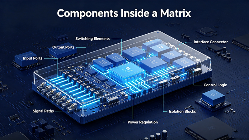
3. Components Inside a Matrix
-
SPnT switches — electromechanical or solid-state switches form the building blocks.
-
Cross-point switch ICs — integrated switch arrays for low-frequency non-blocking matrices.
-
Coaxial cables & harnesses — semi-rigid or flexible cables interconnect switch modules.
-
Control board — microcontroller or FPGA that routes commands to individual switches.
-
Power supply — distributes bias to switches and control logic.
-
Connector panel — SMA, N-Type, or 2.92 mm connectors at the front panel.
-
Termination resistors — 50 Ω terminations for unused paths.
-
Cooling — fans or heat sinks for high-power or dense matrices.
4. Key Specifications
Matrix Size (M × N)
Number of inputs and outputs. Common sizes are 4×4, 8×8, 16×16, 32×32, and beyond.
Frequency Range
Operating band from DC to 40 GHz or higher. Match the matrix to your signal bandwidth.
Loss from input to output. Each switch contributes ~0.2–0.5 dB; more paths means more loss.
Isolation
Signal leakage between active path and inactive paths. Critical for sensitive measurements.
VSWR / Return Loss
Impedance match at all ports. > 15 dB return loss is typical for production matrices.
Switching Speed
Time to reconfigure a path. EM: 10–25 ms; solid-state: < 1 µs.
Power Handling
Maximum RF power per path. Typically 1–10 W CW for solid-state; higher for EM.
Control Interface
Ethernet, USB, GPIB, RS-232, or custom API. Determines ease of integration.
Engineering Note: Cascaded switches add insertion loss. An 8-switch path through a 32×32 matrix can easily accumulate 2–3 dB of total loss — budget accordingly in your link analysis.
5. Typical Applications
-
ATE switching matrices — connecting multiple DUTs to multiple instruments.
-
5G / LTE base station testing — parallel MIMO test of antennas and radios.
-
Satellite payload testing — routing multiple uplink/downlink channels.
-
Antenna range testing — selecting antennas and feeds in OTA chambers.
-
Radar multi-target simulation — assigning threats to receiver channels.
-
Telecom cable / fiber monitoring — OTDR and spectrum analyzer sharing.
-
Quantum computing RF chains — routing microwave pulses between qubits.
-
Defense / EW systems — fast reconfigurable RF front-ends.
6. Selection Checklist
-
Define port count. M inputs × N outputs — include 20–30% growth margin.
-
Choose architecture. Blocking, non-blocking, or hybrid.
-
Verify frequency range. Covers your lowest and highest signal frequency.
-
Calculate insertion loss budget. Each switch adds 0.2–0.5 dB.
-
Confirm switching speed. Manual, EM, or solid-state?
-
Check power handling. Match CW and peak to your application.
-
Verify connector type. SMA, N-Type, BNC, or 2.92 mm.
-
Select control interface. Ethernet, USB, GPIB, or custom.
-
Plan for terminations. 50 Ω terminations for unused ports.
-
Review reliability. MTBF, expected switching cycles, warranty.
Rule of Thumb: For ATE, choose a non-blocking matrix with Ethernet control and > 60 dB isolation. For field-deployable systems, prefer electromechanical switches for higher power handling.
7. Common Pitfalls to Avoid
-
Ignoring cascaded insertion loss. A long switch path loses more signal than the datasheet suggests.
-
Choosing blocking when non-blocking is required. Blocking limits simultaneous paths — check your use case.
-
Underrated isolation. Low isolation contaminates adjacent channels in dense matrices.
-
Ignoring crosstalk. Unused paths act as parasitic antennas at high frequency.
-
Hot-switching EM relays. Damages contacts. Sequence RF off before switching.
-
Mismatched impedance. 50 Ω matrix in a 75 Ω system causes VSWR and loss.
-
Poor cable routing. Tight bends and parallel runs cause crosstalk and stress.
-
Ignoring control latency. Slow control loops delay automated test sequences.
8. Frequently Asked Questions
Q1: What is the difference between an RF switch matrix and an SPnT switch?
An SPnT switch routes one input to one of N outputs. A matrix routes M inputs to N outputs in arbitrary combinations, allowing multiple simultaneous connections.
Q2: What does "blocking" mean in a matrix?
A blocking matrix cannot connect more than one input to a single output. Once a path is set, that output is blocked from other inputs until the path is released.
Q3: How do I scale a matrix to 64×64 or larger?
Use a hybrid architecture — combine multiple smaller non-blocking matrices. Alternatively, use modular expansion with field-replaceable switch cards.
Q4: Are solid-state or electromechanical matrices better?
Solid-state matrices offer microsecond switching and unlimited cycle life, but lower isolation and power handling. Electromechanical matrices deliver best-in-class isolation and RF performance but slower switching.
Q5: Can I control a matrix from Python or LabVIEW?
Yes. Most modern matrices support Ethernet with SCPI, IVI, or LXI protocols. Drivers are available for Python, LabVIEW, MATLAB, and C++.
Q6: How is matrix reliability specified?
Reliability is specified via MTBF (mean time between failures) and per-switch cycle life. Typical EM matrices quote 5–10 million cycles per switch; solid-state matrices have effectively unlimited cycles.
9. Conclusion
The RF switch matrix is the routing backbone of any complex RF system — whether in production test, 5G base station validation, or satellite payload monitoring. Selecting the right matrix comes down to choosing the correct architecture (blocking, non-blocking, or hybrid), matching the frequency range and port count to your application, and budgeting the cascaded insertion loss carefully. By following the checklist and avoiding the common pitfalls above, you can build a matrix that delivers flexible, reliable signal routing for years to come.