






Coaxial Loads and RF Terminations: Types, Power Handling, VSWR, and Selection Guide
A coaxial load is one of the cheapest parts in an RF system and one of the easiest to get wrong. Under-rated, it fails quietly at first — a drifting VSWR, a discoloured connector, a calibration that no longer repeats — and then it fails loudly, usually in the middle of a transmitter test. This guide explains how coaxial loads and RF terminations actually absorb power, how the major types differ, how average and peak ratings are derived and derated, what VSWR and return loss tell you in practice, and how to select a termination that survives your bench.
1. What Is a Coaxial Load?
Every RF source expects to see a defined impedance. A coaxial load provides that impedance at the end of a line: 50 Ω in most commercial, laboratory and cellular systems, 75 Ω in broadcast video, CATV and some telecom infrastructure. Because the load is matched, almost all of the incident wave enters the resistive element and is dissipated as heat; only the small fraction corresponding to the load's reflection coefficient travels back toward the source.
A well-designed termination with 1.10:1 VSWR absorbs about 99.8% of the incident power and reflects roughly 0.2%. A looser 1.50:1 termination absorbs about 96% and reflects 4% — which is still acceptable for protection purposes but is no longer negligible when you are measuring a 1 kW transmitter.
Load, termination, dummy load: three names, one device
The vocabulary is not standardised, but the emphasis differs. Termination describes the function — terminating a line in its characteristic impedance, often at very low power for instrumentation. Load emphasises power absorption and thermal design. Dummy load emphasises substitution: the transmitter is tested into a load instead of an antenna, so no energy is radiated. In practice the three terms are used interchangeably, and a datasheet may call the same part any of them.
Inside the load: where the heat goes
Most coaxial loads share the same four building blocks, and each one sets a different limit on performance:
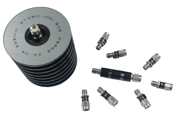
- Resistive element — a thick-film resistor printed on an alumina or beryllium-oxide substrate, or a rod resistor in lower-cost designs. It sets the bandwidth, the VSWR and much of the peak-power limit.
- Dielectric and inner conductor — PTFE, air or a composite dielectric maintains the coaxial geometry. Air-dielectric designs reach higher frequencies; solid dielectric designs are more rugged.
- Body and heatsink — machined aluminium or brass with fins, a cold plate or a water jacket. It sets the average-power rating, because average power is limited by heat removal, not by electrical breakdown.
- Connector interface — N, SMA, 3.5 mm, 7/16 DIN, 4.3-10 and so on. The interface sets the upper frequency limit and, at high power, the peak-power limit.
The thermal chain can be written as a single relationship. Temperature rise above ambient equals dissipated power multiplied by thermal resistance from resistor to ambient:
A 100 W load with R_th = 0.8 °C/W runs 80 °C above ambient at full rating. In a 25 °C room that is already 105 °C at the resistor film — close to the derating limit of many designs, which is why the ambient temperature assumption on the datasheet matters so much.
2. Why RF Terminations Matter in a System
Terminations do four jobs, and each one is a different purchasing decision:
- Equipment protection. Keying a power amplifier into an open or short circuit produces full reflection and can destroy the output stage within microseconds. A load with adequate headroom is the cheapest insurance in the rack.
- Measurement reference. Power meters, spectrum analysers, VNA ports and calibration kits all rely on a known, stable impedance. Metrology-grade terminations specify 1.02:1 to 1.05:1 VSWR precisely because every tenth of a dB of uncertainty propagates into the measurement.
- Absorbing reflected power. Circulators, isolators, hybrid combiners and directional couplers all need a terminated port to dump reverse power safely.
- RF suppression. An unterminated port radiates and leaks. A load keeps the energy inside the chassis, which matters in EMC chambers and multi-channel systems.
3. Types of Coaxial Loads and RF Terminations
Loads are classified three ways — by power class, by mechanical form, and by function — and the three dimensions are largely independent. A 50 W load may be a plug-on SMA, a flange-mount module or a rack panel; the electrical rating does not tell you the form factor you need.
3.1 By power class
- Low power (0.1–2 W): instrumentation terminations for VNA ports, coupler outputs and calibration. Small, precision-machined, often specified to 26.5 GHz or 40 GHz.
- Medium power (5–100 W): air-cooled body with fins; the workhorse of the development bench for amplifier and filter testing.
- High power (100 W–1 kW): finned heatsink or forced air, sometimes with a thermal switch interlock. Used for burn-in, broadcast and base-station testing.
- Very high power (1 kW–100 kW): water- or oil-cooled loads with flow and temperature monitoring, used in transmitter factories, radar depots and high-power RF heating.
3.2 By mechanical form
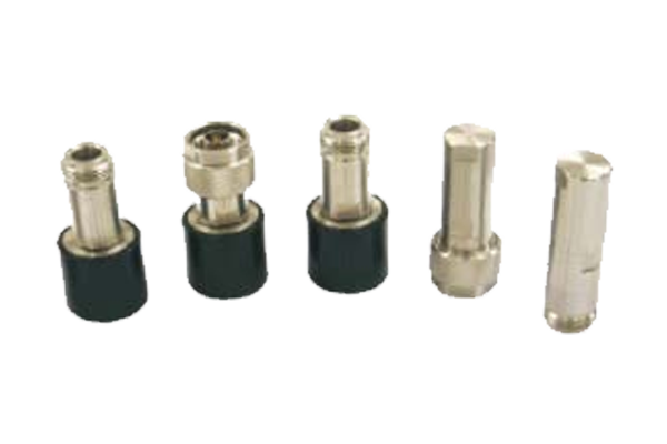
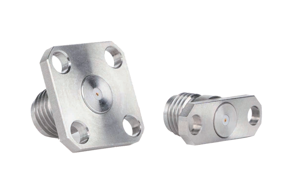
Plug-on terminations mount directly on a connector and rely on the cable or instrument for support. Panel and flange-mount versions bolt to a chassis or cold plate, which is essential above roughly 50 W. Feedthrough (bulkhead) terminations pass through an enclosure wall so the dissipating body sits outside the RF compartment. Module and tray loads integrate several terminations for multi-port test fixtures.
3.3 By function
- Fixed matched load: the default; 50 Ω, broadband, one job.
- Variable or adjustable load: a tunable mismatch used to stress-test amplifiers against real-world antenna conditions and to optimise matching networks.
- Mismatched termination: a load with a defined, repeatable VSWR (for example 2.0:1) used to verify that equipment remains stable under reflection.
- Short and open terminations: not loads in the thermal sense, but standard artefacts in calibration kits and time-domain fault location.
3.4 By connector interface
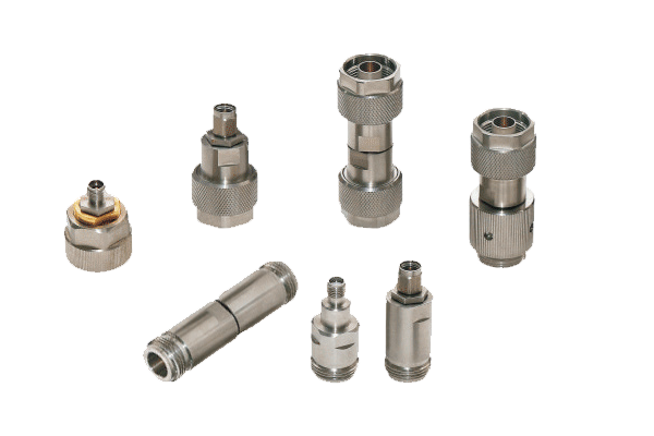
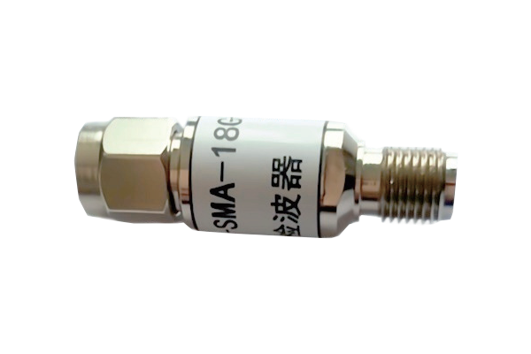
The connector usually decides the frequency ceiling and, above a few hundred watts, the peak-power ceiling as well. SMA is compact and usable to 18 GHz (precision versions to 26.5 GHz) but has limited power capacity and a fragile body. Type N is the general-purpose compromise, usable to 11–18 GHz depending on grade. 7/16 DIN and 4.3-10 were designed for high power and low passive intermodulation in cellular systems; 3.5 mm, 2.92 mm and 1.85 mm are metrology interfaces for 26.5 GHz, 40 GHz and 67 GHz respectively.
| Load type | Typical average power | Typical VSWR | Typical range | Best suited to |
|---|---|---|---|---|
| Precision metrology termination | 0.1–1 W | 1.02:1–1.05:1 | DC–50 GHz+ | VNA calibration, reference standards |
| Low-power plug-on (SMA / N) | 0.5–2 W | 1.10:1–1.20:1 | DC–18 GHz | Port termination, bench measurements |
| Medium-power air-cooled | 5–100 W | 1.15:1–1.30:1 | DC–6 GHz | Amplifier and filter testing |
| High-power heatsink / forced air | 100 W–1 kW | 1.10:1–1.30:1 | DC–3 GHz | Burn-in, broadcast, base station |
| 7/16 DIN or 4.3-10 high power | 50–500 W | 1.10:1–1.25:1 | DC–6 GHz | Cellular, PIM, combiner testing |
| Water- or oil-cooled | 1–100 kW | 1.05:1–1.20:1 | DC–1 GHz | Transmitter factory test, radar |
| Variable / adjustable load | 1–50 W | Adjustable | DC–3 GHz | Mismatch stress testing, matching |
Table 1. Typical figures for orientation only — always confirm against the manufacturer's datasheet for the specific part number.
4. Power Handling: Average, Peak, and What Actually Limits Them
Power ratings are the single most misread line on an RF load datasheet. Two independent limits exist, and they are set by completely different physics.
Average power is a thermal limit
Average power is limited by how fast heat can leave the resistive element. It depends on the substrate, the body mass, the fin area, the airflow and the ambient temperature. A load rated 100 W at 25 °C in free air will not handle 100 W bolted inside a closed rack at 55 °C.
Peak power is a breakdown limit
Peak power is limited by voltage gradient across the dielectric and by arcing at the connector interface. It is independent of heatsinking: a small SMA load may handle 500 W peak but only 1 W average. In pulsed radar and MRI applications, the peak-to-average ratio can exceed 1000:1, and both figures must be satisfied at the same time.
Derating for ambient temperature
Most manufacturers rate the load at 25 °C and derate linearly to zero at a maximum operating temperature — commonly 100 °C to 125 °C at the body. The derating curve, not the headline number, is what you should design against.
| Ambient temperature | Available power (100 W rated at 25 °C) | Derating factor |
|---|---|---|
| 25 °C | 100 W | 100% |
| 50 °C | 75 W | 75% |
| 75 °C | 50 W | 50% |
| 100 °C | 25 W | 25% |
| 125 °C | 0 W | 0% |
Table 2. Linear derating from 25 °C to a 125 °C maximum body temperature. Real curves may be non-linear — read the datasheet.
What VSWR does to power
A load is never perfectly matched, so a small fraction of the incident power is reflected back toward the source. The reflected power is a function of the reflection coefficient:
Γ = (VSWR − 1) / (VSWR + 1)
At 1.20:1, roughly 0.8% of the power returns to the amplifier. That is harmless for the load but not always harmless for the source: reflected power raises junction temperature in the output stage and can trip protection circuits in compact amplifiers. In high-power systems it also creates standing waves on the cable, so the cable and connectors see higher voltage than the forward power alone would suggest.
Altitude, airflow, and duty cycle
Convection-cooled loads lose cooling capacity at altitude because air density falls; manufacturers usually publish a derating curve above about 1500 m. Forced-air loads depend on airflow direction and ducting, and a blocked fin stack can halve the effective rating. Water-cooled loads are limited by inlet water temperature and flow rate, not by ambient air at all — check both, and add a flow switch if the load is unattended.
The headroom rule
Size the load for at least 1.5× the calculated average dissipation, and re-check the number after derating for the real ambient. If the load will run unattended, in a rack, or above 40 °C, 2× is a better starting point than 1.5×. The cost difference between a 100 W and a 200 W load is trivial compared with a destroyed power stage or an invalid measurement campaign.
5. VSWR, Return Loss, and Impedance Match
VSWR and return loss describe the same physical quantity in different units, and both describe how much of the incident wave is reflected. VSWR is the ratio of maximum to minimum voltage on the line; return loss is the reflected power expressed in decibels relative to the incident power.
Return loss (dB) = −20 log₁₀ |Γ|
| VSWR | Return loss | Reflected power | Typical use |
|---|---|---|---|
| 1.02:1 | 40.1 dB | 0.01% | Metrology / calibration standard |
| 1.05:1 | 32.3 dB | 0.06% | Precision instrumentation |
| 1.10:1 | 26.4 dB | 0.23% | Good laboratory load |
| 1.20:1 | 20.8 dB | 0.83% | General-purpose termination |
| 1.30:1 | 17.7 dB | 1.70% | Acceptable for protection only |
| 1.50:1 | 14.0 dB | 4.00% | Marginal for measurement work |
| 2.00:1 | 9.5 dB | 11.1% | Deliberate mismatch / stress test |
| 3.00:1 | 6.0 dB | 25.0% | Fault condition, not a design point |
Table 3. VSWR, return loss and reflected power are three views of the same reflection coefficient.
Two practical rules follow. First, a VSWR specification is only meaningful with a frequency range and a statement of worst case: “1.20:1 maximum, DC–6 GHz” is a specification; “1.20:1 typical” is marketing. Second, the VSWR of a load is not constant across the band — resonances in the resistive element and connector transitions usually appear at the band edges, so always check the sweep, not the mid-band number.
6. Datasheet Specifications to Verify
These are the parameters that decide whether a load survives your application. Anything missing from the datasheet is a question for the supplier.
| Specification | Why it matters | What to check |
|---|---|---|
| Frequency range | Defines the connector and element design | Is it continuous to the top of your band? |
| Impedance | 50 Ω or 75 Ω; a mismatch here invalidates everything else | Match the system, not the instrument's habit |
| VSWR / return loss | Sets measurement uncertainty and reflected power | Maximum, over the full band, at all temperatures |
| Average power | Thermal limit of the load | At what ambient? With what airflow? |
| Peak power | Breakdown limit, relevant to pulsed systems | Pulse width and duty cycle at which it applies |
| Derating curve | Converts the headline rating into a usable one | Slope, maximum body temperature, altitude note |
| Connector interface | Frequency ceiling and mechanical durability | Type, gender, mating cycles, torque spec |
| Cooling requirement | Free convection, forced air or liquid | Mounting orientation, minimum airflow or flow rate |
| Operating temperature | Environmental envelope, not just the resistor limit | Storage and operating range, humidity, IP rating |
| PIM (cellular) | Passive intermodulation in shared-site systems | Specified in dBc at two carriers, typical −150 to −165 dBc |
Table 4. Ten specifications worth confirming before purchase order.
7. Selection Guide in 7 Steps
-
1
Fix the electrical envelope firstFrequency range, impedance and connector type. The connector narrows the catalogue faster than any other decision, and choosing it late usually means compromising on power.
-
2
Calculate the real dissipationTake the worst-case average power the source can deliver, multiply by the absorbed fraction (1 − |Γ|²) for your expected load VSWR, then add margin. Do not use the nominal transmitter rating as the working figure.
-
3
Check peak power separatelyFor pulsed or multi-carrier signals, verify the peak rating at the pulse width and duty cycle you will actually apply. A load that meets the average rating can still arc on peaks.
-
4
Derate for the real environmentUse the ambient inside the rack or enclosure, not the room. Apply the temperature curve, the altitude correction and any airflow restriction before comparing with the datasheet rating.
-
5
Match VSWR to the jobProtection and burn-in tolerate 1.30:1. Power measurement wants 1.10:1 or better. Calibration and VNA work needs 1.05:1 or better, with a certificate.
-
6
Choose the mechanical formPlug-on only below roughly 5 W. Panel or flange mount above that, so the load is supported and heat can leave through the chassis. Feedthrough when the body must sit outside the RF compartment.
-
7
Validate on arrivalSweep the VSWR against a known reference, run the load at rated power for 30–60 minutes with a thermal probe on the body, and log the results. That baseline turns a future failure into a diagnosable event instead of a mystery.
8. Installation and Reliability Notes
- Respect connector torque. Under-torqued connectors raise VSWR and create PIM; over-torqued SMA threads shear. Use a torque wrench and the manufacturer's figure.
- Never hang a load on a cable. Side load on a plug-on termination cracks the dielectric and changes the match. Support the body independently.
- Keep the fins clear. A fin stack blocked by cable bundles loses most of its rating. If the load is in a rack, leave one rack unit of free space above and below.
- Clean and cap connectors. A contaminated interface is the most common cause of a load that “suddenly” measures 1.6:1.
- Monitor water-cooled loads. Interlock on flow, not just temperature; a partial blockage raises the resistor temperature long before the outlet water warms up.
- Log periodic VSWR checks. A 0.1 dB drift in return loss is an early warning of element degradation, long before a visible symptom appears.
9. Typical Applications
The same device serves very different purposes depending on where it sits in the chain: transmitter burn-in and factory acceptance testing; base-station and combiner testing where PIM performance matters as much as power; radar and electronic-warfare benches where peak power dominates the specification; satellite ground stations and VSAT terminals; EMC and immunity testing where energy must be absorbed rather than radiated; semiconductor ATE and device characterisation, where metrology-grade terminations set the uncertainty floor of the whole measurement.
10. Frequently Asked Questions
Both present an impedance to the transmitter, but an antenna radiates the energy while a load converts it into heat. A load is used when radiation is unwanted — during testing, burn-in, or when a port must be terminated to keep the system matched.
You can connect it, but you should not. The 2:1 mismatch reflects about 11% of the power, raises the VSWR seen by the source, and invalidates any measurement made through the load. Use a 75 Ω termination for video, CATV and 75 Ω telecom equipment.
Typically 0.5–2 W average with peak ratings in the hundreds of watts, because SMA is limited by the small dielectric and centre-pin geometry rather than by heatsinking. For sustained power above a few watts, move to a Type N or a panel-mount load with a heatsink.
1.02:1 to 1.05:1 across the specified band, with a traceable certificate and a stated uncertainty. At 1.05:1 the residual reflection contributes about −32 dB, which is small but not always negligible when you are measuring a −30 dB return loss device.
Check three things: the ambient temperature around the fins, the actual duty cycle of the signal (a pulsed source can deliver far more average power than its label suggests), and whether a DC or low-frequency component is present. A load rated for RF may dissipate DC input very differently.
Usually yes. Free-convection ratings assume the body is exposed to still air at 25 °C. Bolted to a chassis inside an enclosure, a 50 W load may only be good for 15–20 W unless the chassis acts as a heatsink or air is moved across the fins.
- Average power is a thermal limit and must be derated for ambient, airflow and altitude; peak power is a breakdown limit and is independent of heatsinking.
- A 1.10:1 load absorbs 99.8% of incident power; a 1.50:1 load reflects 4%. For measurement work, the difference matters.
- The connector, not the resistor, often sets the frequency ceiling and the peak-power ceiling.
- Size for 1.5–2× the calculated dissipation, then verify on arrival with a VSWR sweep and a thermal run.
Technical guide for RF engineers, test-lab managers and procurement teams specifying coaxial loads and RF terminations. Figures are typical values for orientation; confirm every rating against the manufacturer's datasheet for the exact part number before ordering.
About the Author — MeiXun Team
Chief Engineer Wang
High-tech Enterprise, Feifeng Talent
Chief Engineer Wang graduated with a master's degree in high-power microwave from the Institute of Electronics, University of Chinese Academy of Sciences.
View Full Profile- RF Switch Circuit Diagram
- RF Switch
- Ohm's Law
- dBm to Watt
- mW to dBm
- Wavelength to Frequency
- RF Connector
- SMA Connector
- RF Switch Module
- RF Coupler
- RF PIN Switch
- Microwave Coaxial Switch
- PIN Switch
- Coaxial RF Switch
- Waveguide Switch
- Microwave Switch
- Low Noise Amplifier
- PIN Diode Switch
- Coaxial Switch
- RF Microwave Switch
- SPST Switch